The goal of this thesis was to reconstruct realistic hand motions in the presence of noise and occlusions. In the first part of this work, we process multi-view RGB input sequences with off-the-shelf methods to get a robust, but noisy MANO motion estimate. For the second part we split the estimation of the global and local features. As datasets covering both diverse global and local hand motion do not currently exist, we learn the dynamics of the two parts in isolation.
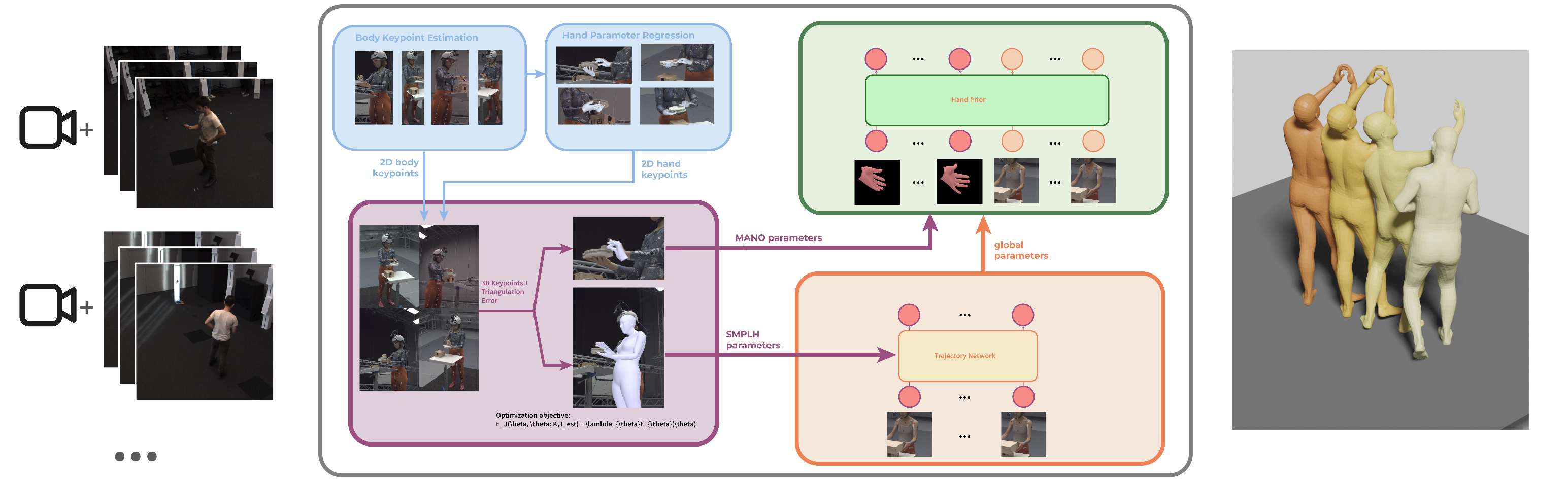
Figure 1: Overview of the proposed solution. The multi-view pipeline reconstructs occlusion-robust hand motion from multi-view input. We leverage HaMeR (blue) to infer body and hand keypoints from monocular images, which are triangulated by minimizing the projection error. Initial MANO parameters are fit to the triangulated keypoints. Our two-stage diffusion model, consisting of the Trajectory Network and Hand Motion Prior refine global and local motion respectively.
Overview
We begin by presenting an overview of our entire pipeline, as illustrated in Figure 1. Our pipeline expects input in the form of RGB image sequences captured from multiple cameras, along with the corresponding camera intrinsics and extrinsics.
In the initial stage, we process the input data to obtain an initial parameteric estimate. For each camera view and frame within the sequence, we employ human detection algorithms to locate bounding boxes around individuals and then identify body keypoints within these bounding boxes. Subsequently, we utilize this information to isolate the bounding boxes encompassing hand regions, providing us with a local estimation of hand articulation. We use HaMeR (Pavlakos, 2019) to regress a sequence of MANO parameters in local space. By backprojecting these MANO estimations, we derive 2D keypoints, which serve as input for triangulating the corresponding 3D keypoints. We refine these 3D keypoints to fit both SMPL-H and MANO parameters, thereby obtaining an initial estimation of hand pose and shape.
In the subsequent phase, we employ two diffusion models to refine the motion estimation derived from the initial optimization-based approaches, aiming to achieve more realistic and plausible representations of hand movements. The SMPL-H initialization is forwarded to the Trajectory Network, which uses a diffusion model to attenuate noise and inconsistencies along the kinematic chain from the hand to the shoulder in order to recover smooth global parameters of the hand. Finally, the enhanced global motion trajectory of the wrist, alongside the refined hand pose estimate, is supplied to the Hand Motion Prior together with the hand estimate to get smooth and plausible motion.
Multi-View Reconstruction
The multi-view reconstruction takes image streams and camera parameters as input and returns a sequence of MANO and SMPL-H parameters for the subject in the scene. Figure 2 shows the single components of the multi-view reconstruction pipeline more closely. We first estimate the 2D keypoints of the body and hand. The keypoints are triangulated by using the camera parameters in order to get the 3D keypoints. Finally, we fit the parameters to the 3D keypoints.
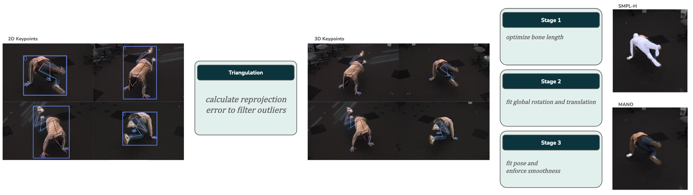
Overview of the multi-view reconstruction pipeline
Keypoint Estimation
The estimation module takes a single image as input and estimates the body and hand keypoints. We employ a top-down approach for the pose detection, which incorporates a person detector first, estimating the location of body parts, and finally calculating the pose for each person. YOLOv5-large (Jocher, 2020) is used to detect all person bounding boxes in each camera view and frame. The cropped bounding boxes serve as input to ViTPose+ (Xu, 2022), which uses a transformer architecture for human pose detection.
Keypoint-based hand detection methods can be very unstable in the presence of occlusions. This is a big factor in the multi-view setting, as the input exhibits large parts of self-occlusion from the subject itself. To this end, we use HaMeR (Pavlakos, 20224) for the keypoint detection. HaMeR uses a transformer-based architecture to regress parameters from image pixels. Its parameter space is $\Theta = {\theta,\beta,\pi}$ , where $\theta$ and $\beta$ are the MANO pose and shape. The parameter $\pi \in \mathbb{R}^3$ corresponds to the translation of the weak camera perspective.
Parts of the training data for HaMeR were annotated with per-joint occlusion mask to improve its robustness. However, the model is not designed to predict occlusion labels. Unlike popular keypoint-based methods that derive proabilities from heatmap predictions, the network also does not provide us with a confidence score.
Keypoint 3D Triangulation
We adpot large parts of the triangulation from EasyMocap. Whenever there are multiple persons in the scene, we need to track and match bounding boxes of the subjects from multiple views. Since the Easymocap methodology requires several parameters, such as tracking distance and bounding box size to be manually tuned, we use a simple Intersection-over-Union tracker to match persons across multiple views and manually correct occuring errors. The bounding box $b_0$ of the initial first frame is manually selected for each view. For each frame $t$, we calculate the valid bounding box $b_t$ as:
\begin{equation} b_t = \max_i \dfrac{\hat{b_t^i} \cap b_{t-1}}{\hat{b_t^i} \cup b_{t-1}}, \end{equation}
where $\hat{b_t^i}$ refers to the i-th bounding box proposal at frame $t$. For a single keypoint, the algorithm uses the Singular-Value-Decomposition (SVD) to find a minimizing point in the 3D space. After the initial candidate position, the 3D point is re-projected to each view to calculate the distance to the input. Outlier views are identified by re-running the triangulation with possible outlier views excluded. Finally, the total reprojection error serves us as a source of confidence for the 3D keypoint location.
Model Fitting
We use a optimization-based approach to transform the 3D keypoints to our parameter space. The opzimization procedure is based on (Joo, 2018) and inspired by EasyMocap, with a focus to unify body and hand information to have noisy but accurate parameter estimates.
The optimization procedure is run two times. Once we minimize the SMPL-H parameters and MANO. Naturally, it would be sufficient to only fit the MANO parameters. However gives us the body additional information in case the hand keypoints are very noisy. By fitting the SMPL-H parameters, we have two sources of global hand parameters (translation $t$, rotation $r$). Fitting only the SMPL-H parameters results in degraded hand articulation due to errors in the shape parameter. The SMPL-H model uses an unified vector $\beta$ for the body and hand shape. Since the changes in the shape parameter can lead to large changes in the finger articulation, the SMPL-H optimized poses often result in bent/straight poses when the shape estimation results in too small/large hands.
In total, we optimize over all MANO parameters of a sequence with $T=60$ frames. For the shape $\beta$ we limit ourselves to 10 parameters. Since the shape of a detected hand is constant, we represent it not over all frames but a 10-dimensional vector.
Based on the authors of MANO, this number serves as a good tradeoff between diversity and space size. Moreover, most datasets we are using also resort to 10 beta values. The optimization pipeline iteratively adds parameters in order to fit ones that have the biggest influence on the joint locations first. As noted in the SMPL paper can the shape be regressed by measuring the bone lengths of the target. To this end, we calculate the per-bone mean over the whole kinematic tree of SMPL. Bone lengths can be very noisy if they were triagulated from a low number of views or from noisy 2D detections. For every bone in the SMPL kinematic tree, we aggregate the minimum triangulation error of the two adjacent joints. To discard faulty measurements, we remove all values where the minimum of the adjacent joints is below the 40% quantile.
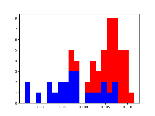
Figure 3: Example of the probability filtering by quantile. Red entries denote valid measurements for the shape parameter fitting while blue measurements are discarded.
First of all, we present an overview of the losses used during the optimization:
\begin{equation} L_{\text{vel}} = ||\dot{x} - \dot{x_0}||_2 \end{equation}
\begin{equation} L_{\text{accel}} = ||\ddot{x}||_2 \end{equation}
\begin{equation} L_{\text{initial}} = ||p - p_{\text{prev}}||_2 \end{equation}
\begin{equation} L_{\text{kp3d}} = ||x - FK(\theta,\beta,t)||_2 \cdot c \end{equation}
\begin{equation} L_{\text{kp2d}} = ||x_{2D} - \Pi_{\text{cam}} FK(\theta,\beta,t)||_2 \cdot c \end{equation}
\begin{equation} L_{\text{reg}} = ||x - x_0||_2 \end{equation}
\begin{equation} L_{\text{regs}} = ||\beta - \beta_0||_2 \end{equation}
First of all, the global translation $T$ and rotation $R$ are estimated with: \begin{equation} L_{global} = \lambda_{\text{kp3d}} L_{\text{kp3d}} + \lambda_{\text{vel}} L_{\text{vel}}, \end{equation}
where $\lambda_{\text{kp3d}} = 1$ and $\lambda_{\text{vel}} = 1$. EasyMocap optimizes over axis-angle rotations for the pose $\theta$, which is not a continuous representation and thus is prone to twisting and orientation artifacts of the body, which requires regulation of velocities and acceleration. Since we are not recovering the body pose, our methods rely on smooth and accurate SMPL-H body parameters. In the first step, we optimize the body with: \begin{equation} \lambda_{\text{kp3d[body]}} = 1, \lambda_{\text{reg}} = 0.1, \lambda_{\text{regs}} = 0.1 \end{equation} The shape regularization prevents the optimizer from generating extreme body shapes to fit the keypoints, while the pose regularization prevents the movement of joints that are typically at zero and difficult to capture with the joint-based representation.
We continue by fitting the hand: \begin{equation} \lambda_{\text{kp3d[body]}} = 1, \lambda_{\text{kp3d[hand]}} = 5, \lambda_{\text{reg}} = 0.1, \lambda_{\text{regs}} = 0.01, \end{equation} These steps are separate in order to prevent local minima in the elbow by correcting errors in the shape. At this point there exists an accurate but noisy estimate, which is smoothed in the subsequent optimization routine with:\ \begin{equation} \lambda_{\text{kp3d[body]}} = 1, \lambda_{\text{kp3d[hand]}} = 5, \lambda_{\text{reg}} = 0.1, \lambda_{\text{regs}} = 0.01, \lambda_{\text{vel}} = 0.01, \lambda_{\text{acc}} = 5, \end{equation} Additionally, velocity and acceleration are enforced on the parameters aswell. Finally, we fit the 2D keypoints with strong regularization on the initial pose and smoothness:
\begin{equation} \lambda_{\text{initial}} = 1, \lambda_{\text{regs}} = 0.1, \lambda_{\text{kp2d}} = 0.01 \end{equation}
For the MANO optimization, we employ a similar procedure. We omit the body 3D keypoint loss. Furthermore, we reduce velocity and acceleration weights to $\lambda_{\text{vel}} = 0.0001$ and $\lambda_{\text{acc}} = 0.0001$.
The optimization is performed using the L-BFGS [LiuN89] optimizer with learning rate of 1, a maximum of 10 iterations and the wolfe line search function of the pytorch package.
Hand Motion Processing
In this section, the approach to our diffusion-based hand motion prior is described. The goal is to refine the optimization-based results from the multi-view pipeline in order to reconstruct smooth and plausible motion. While the optimization could incorporate regularizing losses, plausible motion cannot be enforced. We supply the hand motion prior with the noisy multi-view output. Global and local motion are separated in order to leverage a wider range of datasets for the task, as stated at the beginning of the chapter. We noticed that learning both global and local features together raised some issues. The Trajectory Network predicts the global dynamics of the hand based on the detections of the body. The Hand Motion Prior learns the local hand pose from the global features of the Trajectory Network and the estimate of the multi-view pipeline. The two parts follow a unified approach and architecture which is why we will cover the two diffusion models in parallel.
Data Representation
We represent the Trajectory Network body motion sequence G as a tuple $g_n = (\gamma_G,\Phi_G,\theta_G,\beta_G,J_G)$ for every frame $n$ in the sequence.
\begin{equation} \gamma_G \in \mathbb{R}^3,\ \Phi_G \in \mathbb{R}^{2\times 3},\ \beta_G \in \mathbb{R}^{10},\ \theta_G \in \mathbb{R}^{42\times 3},\ J_G \in \mathbb{R}^{25\times 3},\ \end{equation}
For each frame in the sequence, all features are concatenated to a feature vector. We expand the shape parameter to a size of (T,4,3) by repeating the values for every frame and pad the values in order to make the input divisible by three. This gives us a final size of (T,73,3). For experiments with alternative representations, we refer to the appendix.
\paragraph{Hand Motion Prior} The hand motion sequence $L$ for the Hand Motion Prior is represented as a tuple $l_n = (\gamma_L,\Phi_L,\theta_L,\beta_L,J_L)$ for every frame $n$ in the sequence.
\begin{equation} \gamma_L \in \mathbb{R}^3\ \Phi_L \in \mathbb{R}^{2\times 3}\ \beta_L \in \mathbb{R}^{10}\ \theta_L \in \mathbb{R}^{30\times 3}\ J_L \in \mathbb{R}^{21\times 3}\ \end{equation}
We concatenate the features the same way as described in the above paragraph.
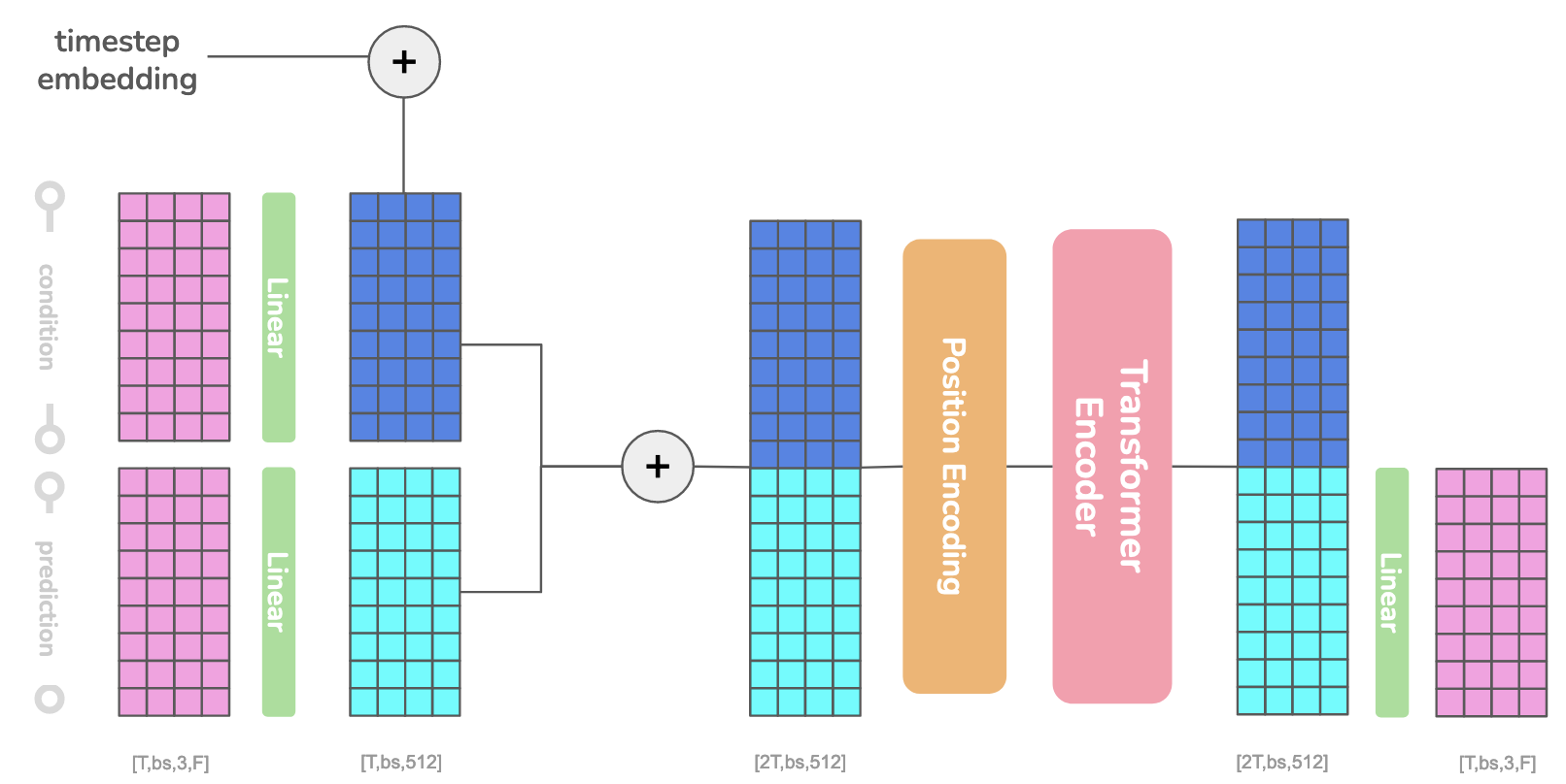
Architecture of the Trajectory Network and Hand Motion Prior. (F) denotes the number of input features, (T) the number of frames in the sequence.
Network Definition
We train a denoiser $D_G(\cdot)$ to recover smooth arm motion $\hat{G_0}$ from whole body inputs $\tilde{G}$: \begin{equation} \hat{G_0} = D_G(G_t,t,\tilde{G}). \end{equation} $\tilde{G}$ denotes the noisy body pose, which is supplied either from the data augmentation during training or from the multi-view pipeline during evaluation. $t$ denotes the sampled diffusion timestep. While the body pose serves as a conditioning input, we only consider the shoulder, elbow and wrist rotations. From the denoised $\hat{G_0}$ we extract the wrist translation $\gamma_G$ and wrist rotation $\Phi_G$ as input to the Hand Motion Prior.
\paragraph{Hand Motion Prior} We follow a similar definition for the Hand Prior denoiser $D_L(\cdot)$: \begin{equation} (\hat{L_0},\hat{R_0}) = D_L((L_t,\hat{R_0}),t,(\tilde{L},\gamma_G,\Phi_G)). \end{equation} where we predict the smooth hand pose $\hat{L_0}$. The denoised wrist translation $\gamma_G$ and wrist rotation $\Phi_G$ serve as conditioning signal.
Data Augmentation
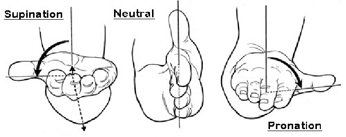
Supination and pronation are movements of the elbow that influence the global hand rotation without affecting the translation. Image taken from Vetrice et al. (2017).
During training on ground truth motion datasets, we apply synthetic noise and occlusion masks in order to simulate noisy inputs from the multi-view pipeline. \paragraph{Trajectory Network} During training, we add noise to the arm and wrist poses. The noise follows a normal distribution with $\mu = 0$. For the upper arm, we add $\sigma_{UA} = 0.01$, the lower arm $\sigma_{LA} = 0.04$ and wrist $\sigma_{WR} = 0.06$. Additionally, we add noise to the elbow rotation controlling the supination and pronation of the hand. These are rotations of the elbow that control the global orientation of the hand without affecting the translation (see figure 5. This step is crucial, as optimization-based fitting frequently introduces errors along this axis, as we have empirically observed from the optimization results. We mask the input with a mask based on the fitting error generated by the optimization-based pipeline. As a further data augmentation step, we employ synthetic occlusion masks to train the model in the task of motion infilling. Since occlusions usually persist over multiple consecutive frames rather than single frames, we remove high frequency noise from our masks by applying a gaussian filter over a random binary sequence and thresholding to get the mask. The process is illustrated in Figure 6.
In the multi-view results, we visually observed correlations between the wrist position accuracy and the accuracy of hand detections obtained by the triangulation. We mask out a frame whenever one of three criteria is satisfied: \begin{equation} \Big(\dfrac{1}{n}\sum_n \mathcal{P}(J^i_{\text{hand}})\Big) < 0.3 \end{equation} \begin{equation} \Big(\sum_n \mathcal{P}(J^i_{\text{hand}}) < 0.3\Big) < 8 \end{equation} \begin{equation} \mathcal{P}(J^i_{\text{wrist}}) < 0.7 \end{equation}
\paragraph{Hand Motion Prior} We add Gaussian noise to all poses $\theta$ as an augmentation step to generate synthetic input data. Since errors occur in different scenarios such as we try to model those as well. We introduce three noise scales which ideally correspond to (1) small triangulation inaccuracies, (2) unobserved occlusions and (3) triangulation of outlier detections.
- we create a mask with $\mathcal{P}(\text{mask}) = 70%$ and add normal noise with $\mu = 0$ and $\sigma = 0.06$
- we create a mask with $\mathcal{P}(\text{mask}) = 40%$ and add normal noise with $\mu = 0$ and $\sigma = 0.15$
- we create a mask with $\mathcal{P}(\text{mask}) = 10%$ and add normal noise with $\mu = 0$ and $\sigma = 0.2$

Example creation of a synthetic mask. Random input (top row) is smoothed with a Gaussian kernel (middle) and tested against a threshold to obtain a binary mask (bottom).
The masks are created with the same procedure as described in the above paragraph. Finally, the noisy joint positions are obtained by calculating the forward kinematics of the noisy parameters.\
Architecture
Both diffusion models adopt the transformer encoder structure from MDM (Tevet,2023), with respective motion representation. The input representation is reshaped such that all features have the size $(T \times d \times 3)$ where $d$ represents the number of data fields. We split 6D rotation features into $(2 \times 3)$ matrices and pad the shape $\beta$ to bring it into the shape $(4 \times 3)$. The input is flattened and passed through a linear layer, which returns the latent feature representation with size $(T \times bs \times 512)$ where $bs$ denotes the batch size and 512 our used latent size.
The conditional input is processed with the same procedure, but uses its own linear layer to bring the features into latent representation. A temporal embedding of the current timestep is projected to the transformer dimension and added to the conditional input. It consists of a positional encoding of the current sampled timesteps, which is passed through two linear layers with a SiLU activation function in between. Together with the latent vector from the input, the conditional embedding is concatenated to our transformer input of size $(2T \times bs \times 512)$. We pass the data through a positional encoding to encode the temporal nature of our data, which is preceded by a transformer encoder. The output condition is removed from the transformer output and a linear layer transforms the data from its latent size back to the input motion representation.
Data Normalization
Normalization is an essential step to help the model learn the dynamics of the motion more efficiently. We follow the literature (Guo et al., 2022) and preprocess each sequence to bring them into a canonicalized representation.
Trajectory Network
Following Guo et al. (2022), we apply forward kinematics to position the subject on the ground plane. As each subject possesses unique shape values influencing the height of the SMPL-H root $H$, we initialize the translation of the first frame to $(0,0,H)$. The global rotation $\Phi$ of the first frame is set to the canonical rotation $\bar{\Phi}_0$, which points forward along the xy-axes. We normalize the sequence by multiplying the inverse of the canonical rotation:
$$ \bar{\Phi} = \Phi \cdot (\Phi^{-1} \cdot \bar{\Phi}_0) $$
Since SMPL-H translates the model with respect to the global orientation, we also need to transform the global translation accordingly:
$$ \bar{\gamma} = \gamma \cdot (\Phi^{-1} \cdot \bar{\Phi}_0) $$
We calculate normalization metrics on the AMASS data by calculating the mean and variance over all clips. Due to the low coverage of shape values, we don’t perform the normalization for the shape parameter $\beta$.
Hand Motion Prior
We apply the normalization process to the MANO sequence as well. The wrist root joint is placed at the origin of the coordinate frame and the direction of the initial frames is canonicalized to the identity rotation $\mathcal{I}$. Consequently, we apply the equations above with $\bar{\Phi}_0 = \mathcal{I}$.
To achieve a canonical representation of the joints, we employ forward kinematics on the MANO parameters. The design of the MANO shape parameter does not align the root joint to the origin, which is why we subtract the offset induced by the shape parameter.
Similarly to the approach adopted for body sequences, we normalize the input using the mean and variance of the dataset. Despite the datasets exhibiting significant diversity in global and local motion, we calculate the mean and variance across all datasets.
Training
We train our denoiser $D_G(\cdot)$ using $L_{\text{simple}}$ as defined in Ho et al. (2020), and additionally regularize the drift of the wrist due to multiple rotations with a 3D joint loss ($L_{\text{wrist}}$). We define $\tilde{J} = J_{\tilde{G}}$ and $J’ = J_{G_0}$.
To mitigate drift caused by the multiplication of rotation matrices in the kinematic chain, we obtain the wrist and arm joint positions $J_{\text{WA}}$ by applying forward kinematics:
$$ J_{\text{WA}} = FK(\tilde{J})_{\text{WA}} $$
$$ J_0 = FK(J’)_{\text{WA}} $$
The loss is only taken over the wrist:
$$ L_{\text{wrist}} = | J_0 - J_{\text{WA}} |^2 $$
where $G_0$ refers to the ground-truth motion and $\tilde{G}$ to the noisy body input. Furthermore, we add velocity and acceleration smoothness losses:
$$ L_{\text{vel}} = | \dot{J_0} - \dot{J}_{\text{WA}} |^2 $$
$$ L_{\text{acc}} = | \ddot{J}_0 |^2 $$
The overall loss is defined as:
$$ L = L_{\text{simple}} + \lambda_{\text{wrist}} L_{\text{wrist}} + \lambda_{\text{vel}} L_{\text{vel}} + \lambda_{\text{acc}} L_{\text{acc}} $$
During training, we augment our data to synthetically generate $\tilde{G}$ as described in Section Augmentation.
The trajectory network is trained for 100k iterations using the Adam optimizer with a learning rate of $1 \times 10^{-4}$. The batch size is set to 32 and the latent size to 512. The weights for loss terms are set as follows: $\lambda_{\text{acc}} = 1$, $\lambda_{\text{vel}} = 1$, and $\lambda_{\text{wrist}} = 1$.
Hand Motion Prior
We train our denoiser $D_L(\cdot)$ using the simplified denoising loss $L_{\text{simple}}$ (as in Ho et al., 2020), and additional losses over the reconstructed joints:
$$ J_{\text{RC}} = FK(\tilde{L}_{\text{joints}}) $$
We compute the L2 loss over the reconstructed joints:
$$ L_{\text{3D}} = | J_L(L_0) - J_{\text{RC}} |^2 $$
We also apply the same velocity and acceleration smoothness losses:
$$ L_{\text{vel}} = | \dot{J}_W(L_0) - \dot{J}_W(\tilde{G}) |^2 $$
$$ L_{\text{acc}} = | \ddot{J}_W(L_0) |^2 $$
Here, $G_0$ refers to the ground-truth motion and $\tilde{L}$ to the noisy body input.
The overall loss is defined as:
$$ L = L_{\text{simple}} + \lambda_{\text{3D}} L_{\text{3D}} + \lambda_{\text{vel}} L_{\text{vel}} + \lambda_{\text{acc}} L_{\text{acc}} $$
During training, we augment our data to synthetically generate $\tilde{L}$ as described in Section Augmentation.
The hand motion prior is trained for 60k iterations using the Adam optimizer with a learning rate of $1 \times 10^{-4}$. The batch size is 64 and the latent size is 512. Loss weights are: $\lambda_{\text{acc}} = 1$, $\lambda_{\text{vel}} = 1$, and $\lambda_{\text{3D}} = 50$.
Inference
During inference, we normalize the observations with the same procedure as the synthetic data. We perform 1000 denoising diffusion steps for both models.